Getting Started with EdgeLab on Local PC

1. Prerequisites

Please prepare the following

Grove - Vision AI Module or SenseCAP A1101
USB Type-C cable
Linux PC

2. Configure host environment

We first need to configure the host PC. Here we have used a PC with Ubuntu 22.04 installed.

Step 1. Clone the following repo and access it

git clone https://github.com/Seeed-Studio/Edgelab
cd Edgelab

Step 2. Configure the host environment by running the following script which will download and install the relevant dependencies

python3 tools/env_config.py

The above script will mainly install PyTorch, MMCV, MMClassification, MMDetection and MMPose.

Note: The above script will add various environment variables to the file ~/.bashrc, establish a conda virtual environment called edgelab, install relevant dependencies inside the virual environment.

Step 3. Eventhough everything is initialized at this point, they are not activated. Activate conda, virtual environments, and other related environment variables

source ~/.bashrc
conda activate edgelab

Now we have finished configuring the host environment

3. Generate firmware image

We need to generate a firmware image for the Grove - Vision AI to support the analog meter reading detection model because the default firmware which is pre-installed out-of-the-box does not support it.

Analog meter reading detection

If you want to download an already pre-compiled firmware, please follow the links below. But we recommend you to compile the firmware from source, so that you will have the latest firmware always.

Grove - Vision AI Module
SenseCAP A1101

Step 1: Download GNU Development Toolkit

cd ~
wget https://github.com/foss-for-synopsys-dwc-arc-processors/toolchain/releases/download/arc-2020.09-release/arc_gnu_2020.09_prebuilt_elf32_le_linux_install.tar.gz

Step 2: Extract the file

tar -xvf arc_gnu_2020.09_prebuilt_elf32_le_linux_install.tar.gz

Step 3: Add arc_gnu_2020.09_prebuilt_elf32_le_linux_install/bin to PATH

export PATH="$HOME/arc_gnu_2020.09_prebuilt_elf32_le_linux_install/bin:$PATH"

Step 4: Navigate to the following repo of Edgelab

cd Edgelab/examples/vision_ai

Step 5: Download related third party, tflite model and library data (only need to download once)

make download

Step 6: Compile the firmware according to your hardware

For Grove - Vision AI Module

make HW=grove_vision_ai APP=meter
make flash

For SenseCAP A1101

make HW=sensecap_vision_ai APP=meter
make flash

This will generate output.img inside ~/Edgelab/examples/vision_ai/tools/image_gen_cstm/output/ directory

Step 7: Generate firmware image firmware.uf2 file so that we can later flash it directly to the Grove - Vision AI Module/ SenseCAP A1101

python3 tools/ufconv/uf2conv.py -t 0 -c tools/image_gen_cstm/output/output.img -o firmware.uf2

This will generate firmware.uf2 inside ~/Edgelab/examples/vision_ai directory

Object Detection

Firmware generation for object detection model will be coming soon!

4. Prepare dataset

Analog meter reading detection

With existing dataset

We have already prepared a ready-to-use dataset for your convenience

Step 1. Click here to download the dataset
Step 3. Create a new folder named datasets inside the home directory

cd ~
mkdir datasets

Step 3. Unzip the previously downloaded dataset and move the meter folder into the newly created datasets folder

With your own dataset

Here we explain how to use your own dataset

Collect dataset

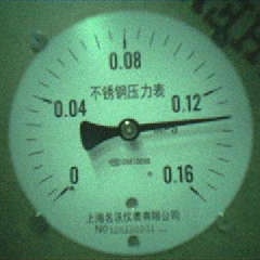
If you want to train your own analog meter detection model for a specific application, you need to spend sometime to collect images to prepare a dataset. Here you can take several photos (start with 200 and go higher to improve accuracy) of the analog meter that you want to detect with the meter pointer at different points and also take photos at different lighting conditions and different environments as follows

Pointer reading at dark environment

Pointer reading at light environment

Annotate dataset

Next we need to annotate all the images that we have collected. Here we will use an application called labelme which is an open source image annotation tool.

Step 1. Visit this page and install labelme according to your operating system
Step 2. On the command-line, type the following to open labelme

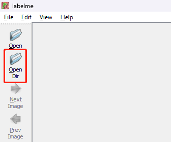
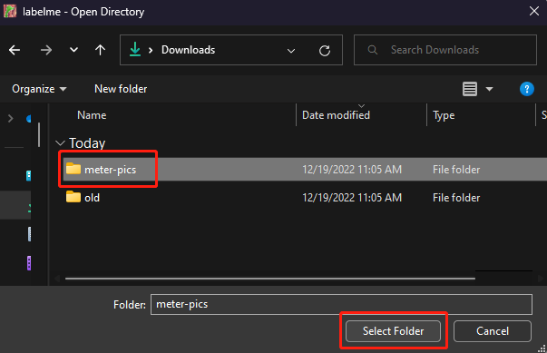
labelme

Step 3. Once labelme opens, click on OpenDir, select the folder that you have put all the collected images and click Select Folder

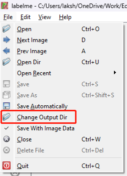
Step 4. Later, when we annotate images, labelme will generate a json file for each image and this file will contain the annotation information for the corresponsing image. Here we need to specify a directory to store these image annotations because we recommend to store these json files and image files in 2 different folders. Go to File > Change Output Dir

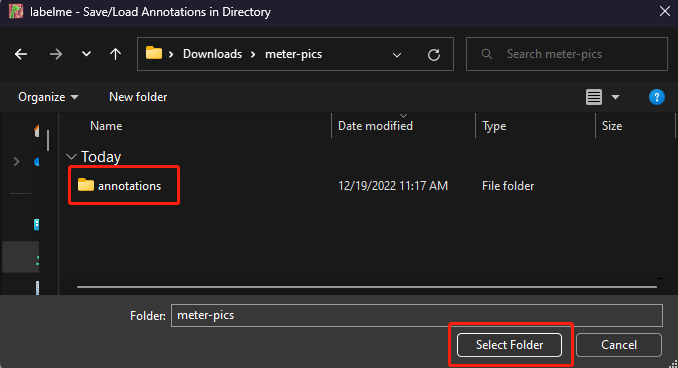
Step 5. Create a new folder, select the folder and click Select Folder

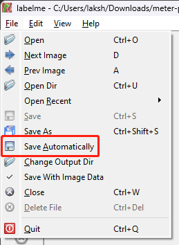
Step 6. Go to File > Save Automatically to save time when annotating all the images. Otherwise it will pop up a prompt to save each image.

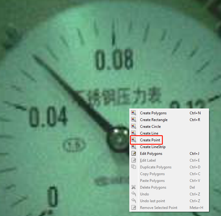
Step 7. Right click on the first opened image and select Create Point

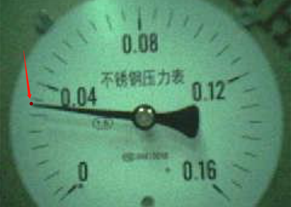
Step 8. Draw a point at the tip of the pointer, set any label name and click OK

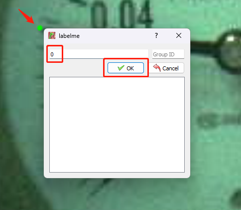
After the point, there will be a new json file created automatically for each image file under "annotations" folder as mentioned before.

Organize dataset

Now you need to manually organize the dataset by splitting all the images and annotations into train, val, test directories as follows

Here we recommend you to split in the following percentages

train = 80%
val = 10%
test = 10%

So for example, if you have 200 images, the split would be

train = 160 images
val = 20 images
test = 20 images

meter_data
    |train
        |images
            |a.jpg
            |b.jpg
        |annotations
            |a.json
            |b.json
    |val
        |images
            |c.jpg
            |d.jpg
        |annotations
            |c.json
            |d.json
    |test
        |images
            |e.jpg
            |f.jpg
        |annotations
            |e.json
            |f.json

Object detection

With public dataset

You can use public datasets to easily start training

Use PASCAL VOC dataset

We have already configured yolov3_mbv2_416_coco.py file out-of-the-box to download and include the PASCAL VOC dataset which is a public dataset.

Use other public datasets

You can also use other public datasets available online. Simply search open-source datasets on Google and choose from a variety of datasets available. Make sure to download the dataset in COCO or Pascal VOC format because only those 2 formats are supported by training at the moment.

Here we will demonstrate how to use Roboflow Universe to download a public dataset ready for training. Roboflow Universe is a recommended platform which provides a wide-range of datasets and it has 90,000+ datasets with 66+ million images available for building computer vision models.

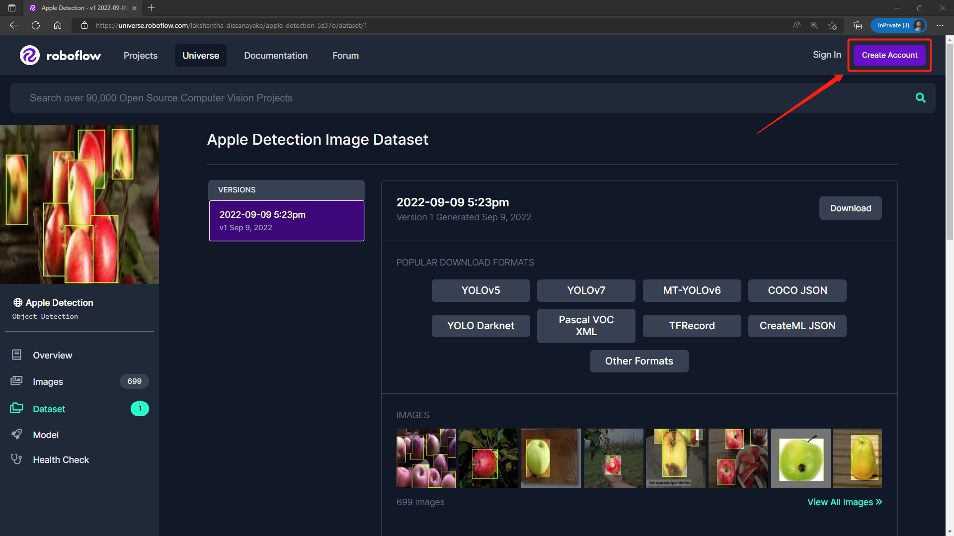
Step 1. Visit this URL to access an Apple Detection dataset available publicly on Roboflow Universe. This is a dataset with a single class named as apple
Step 2. Click Create Account to create a Roboflow account

Step 3. Click Download, select COCO as the Format, click download zip to computer and click Continue

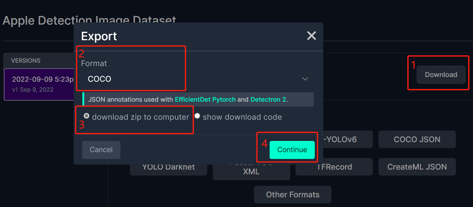
Note: You can also choose Pascal VOC as the Format

This will place a .zip file in the Downloads folder on your PC

Step 4. Go to Downloads folder and unzip the downloaded file

cd ~/Downloads
unzip **file_name.zip**

## for example
unzip Apple\ Detection.v1i.coco.zip

With your own dataset

You can use your own dataset to easily start training

If you use your own dataset, you will need to annotate all the images in your dataset. Annotating means simply drawing rectangular boxes around each object that we want to detect and assign them labels. We will explain how to do this using Roboflow.

Here we will use a dataset with images containing apples

Step 1. Click here to sign up for a Roboflow account
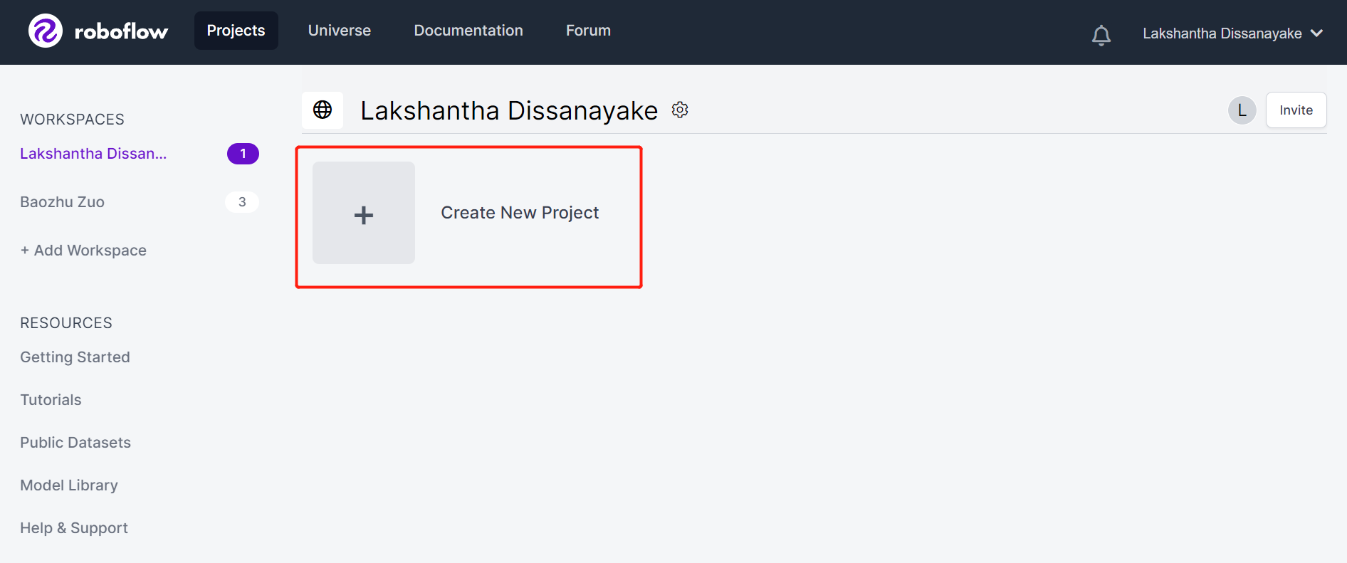
Step 2. Click Create New Project to start our project

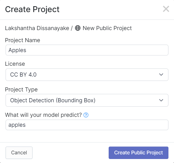
Step 3. Fill in Project Name, keep the License (CC BY 4.0) and Project type (Object Detection (Bounding Box)) as default. Under What will your model predict? column, fill in an annotation group name. For example, in our case we choose apples. This name should highlight all of the classes of your dataset. Finally, click Create Public Project.

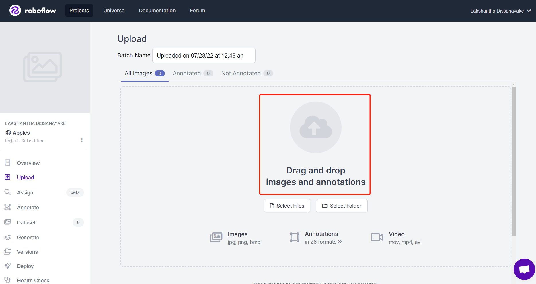
Step 4. Drag and drop the images that you have captured

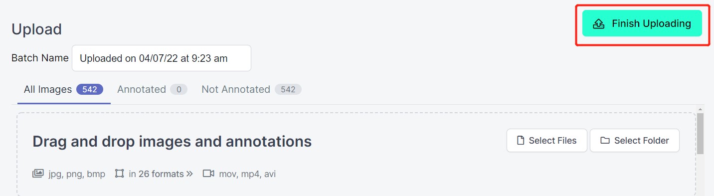
Step 5. After the images are processed, click Finish Uploading. Wait patiently until the images are uploaded.

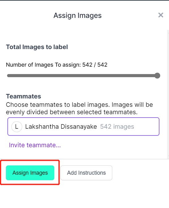
Step 6. After the images are uploaded, click Assign Images

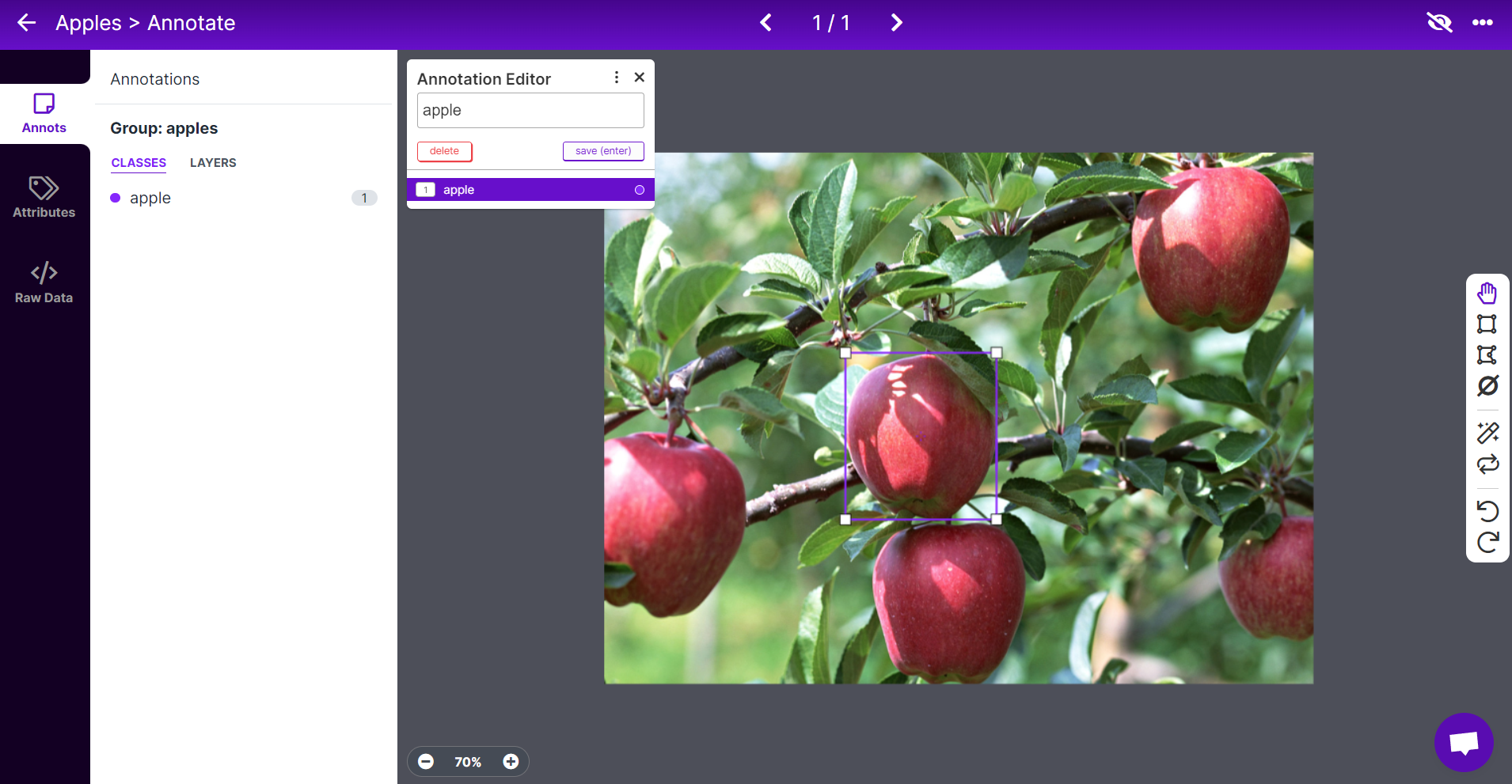
Step 7. Select an image, draw a rectangular box around an apple, choose the label as apple and press ENTER

Step 8. Repeat the same for the remaining apples

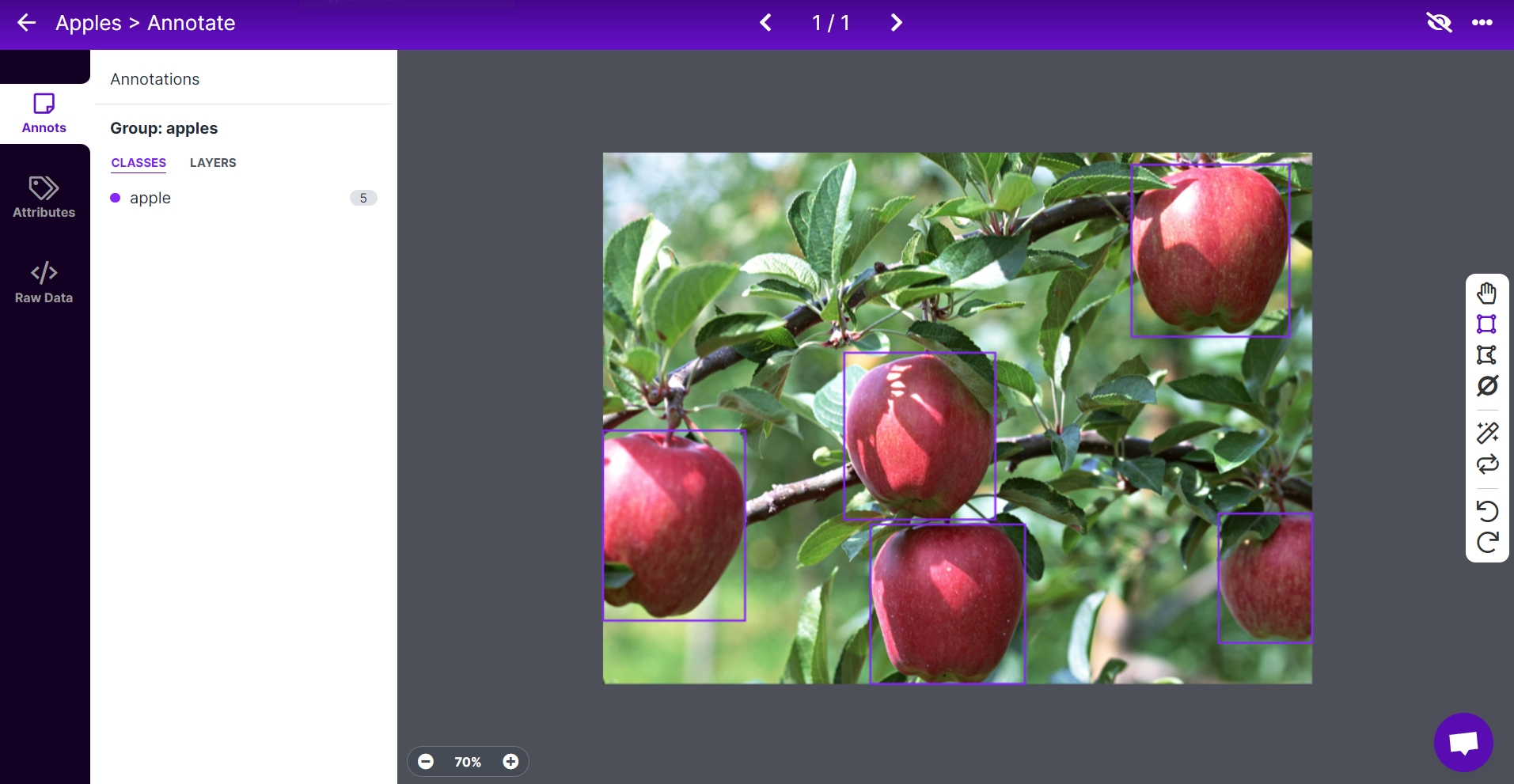
Note: Try to label all the apples that you see inside the image. If only a part of an apple is visible, try to label that too.

Step 9. Continue to annotate all the images in the dataset

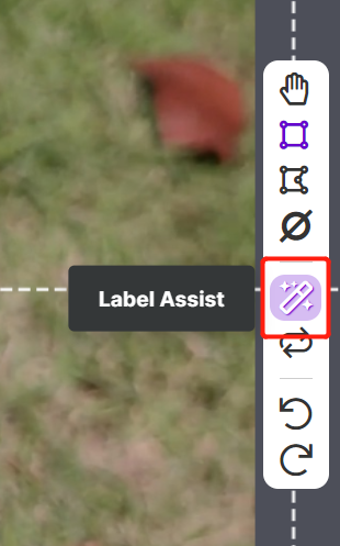
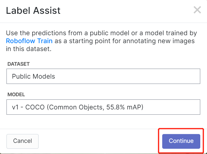
Roboflow has a feature called Label Assist where it can predict the labels beforehand so that your labelling will be much faster. However, it will not work with all object types, but rather a selected type of objects. To turn this feature on, you simply need to press the Label Assist button, select a model, select the classes and navigate through the images to see the predicted labels with bounding boxes

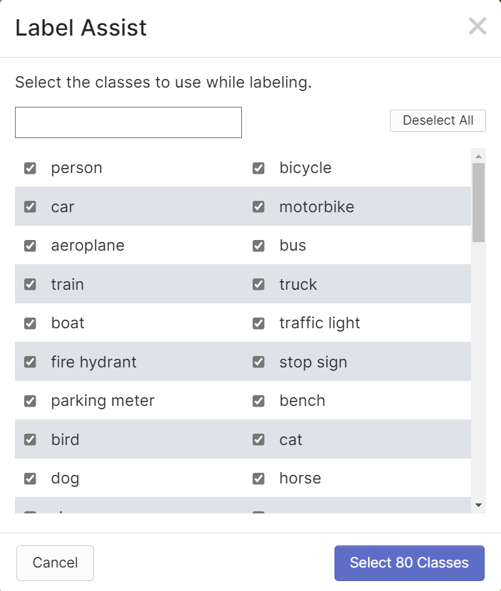
As you can see above, it can only help to predict annotations for the 80 classes mentioned. If your images do not contain the object classes from above, you cannot use the label assist feature.

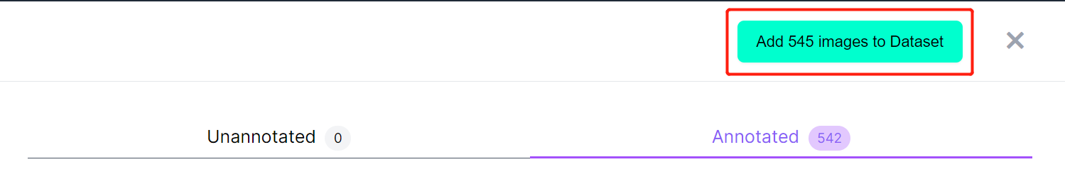
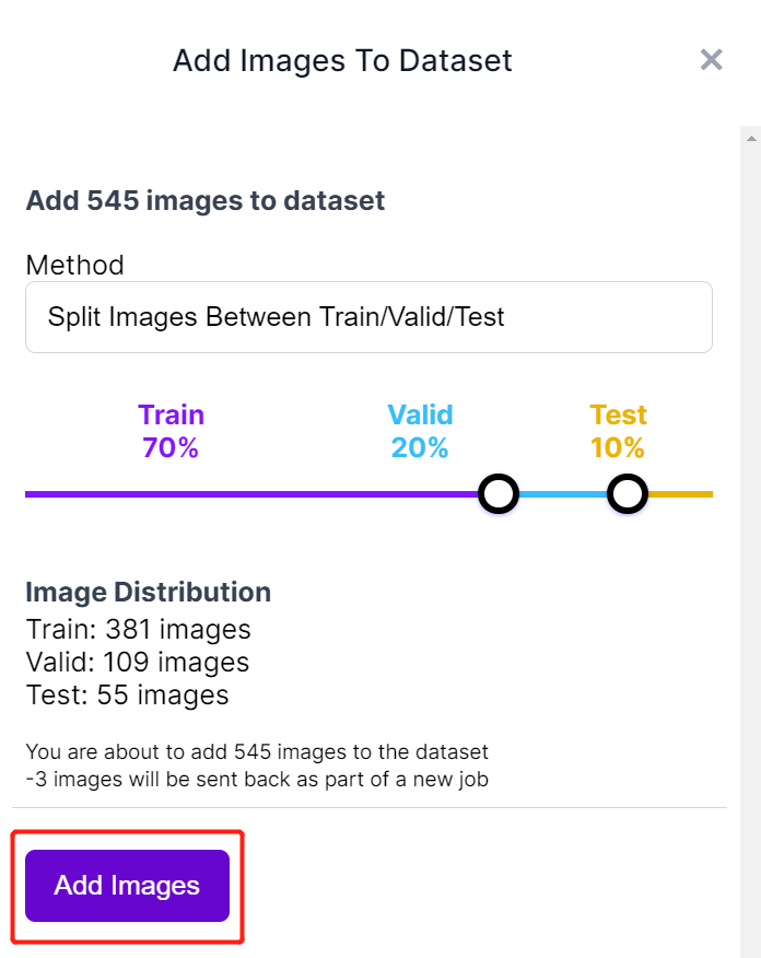
Step 10. Once labelling is done, click Add images to Dataset

Step 11. Next we will split the images between "Train, Valid and Test". Keep the default percentages for the distribution and click Add Images

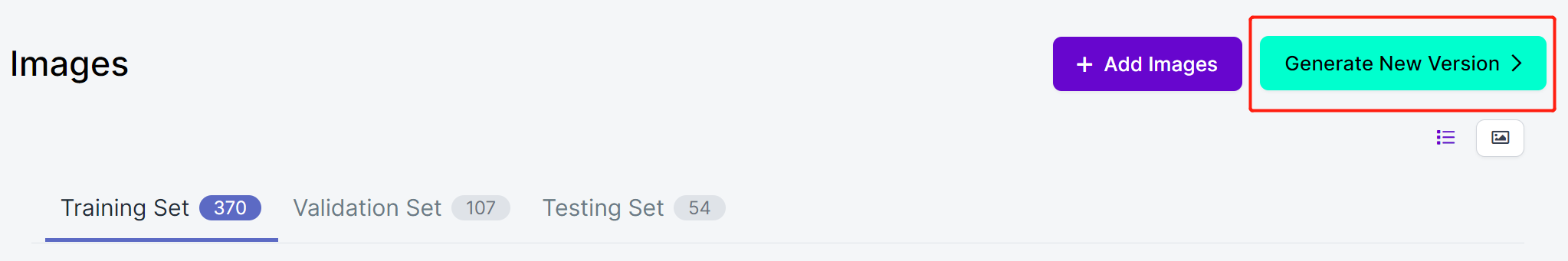
Step 12. Click Generate New Version

Step 13. Now you can add Preprocessing and Augmentation if you prefer
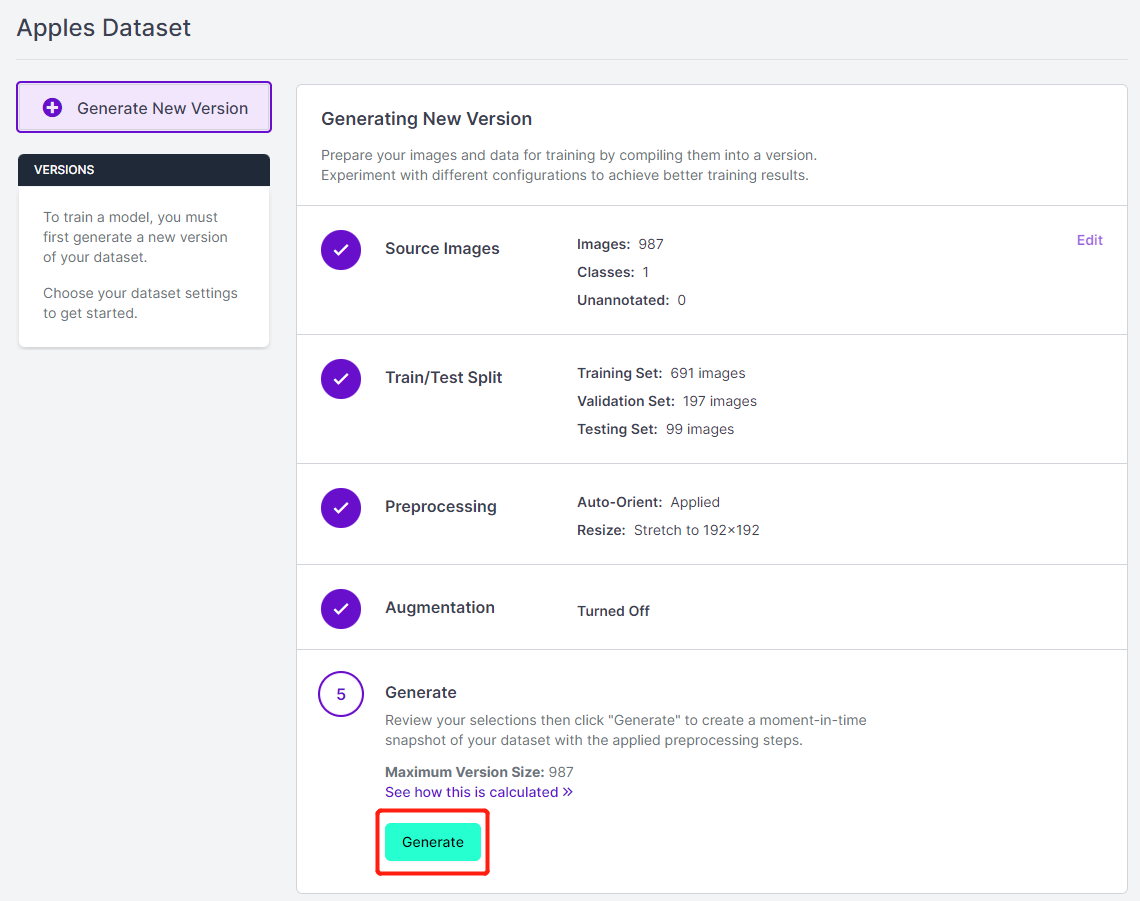
Step 14. Next, proceed with the remaining defaults and click Generate

Step 15. Click Download, select COCO as the Format, click download zip to computer and click Continue

Note: You can also choose Pascal VOC as the Format

This will place a .zip file in the Downloads folder on your PC

Step 16. Go to Downloads folder and unzip the downloaded file

cd ~/Downloads
unzip **file_name.zip**

## for example
unzip Apple\ Detection.v1i.coco.zip

5. Start training

Here we provide instructions on how to train AI models for object detection and analog meter reading detection.

Configuration file

We will choose the profile according to the task that we want to implement. We have prepared preconfigured files inside the the configs folder.

For our meter reading detection example, we will use pfld_mv2n_112.py config file. This file will be mainly used to configure the dataset for training including the dataset location.

For our object detection example, we will use yolov3_mbv2_416_voc.py config file. This file will be used to configure the dataset for training including the dataset location, number of classes and the label names.

Analog meter reading detection

With existing dataset

Here we use the previously downloaded dataset for training

Execute the following command inside the activated conda virtual environment terminal to start training an end-to-end analog meter reading detection model.

python tools/train.py mmpose configs/pfld/pfld_mv2n_112.py --gpus=1 --cfg-options total_epochs=100

The format of the above command looks like below

python tools/train.py <task_type> <config_file_location> --gpus=<cpu_or_gpu> --cfg-options total_epochs=<number_of_epochs>

where:

<task_type> refers to either mmcls for classfication, mmdet for detection and mmpose for pose estimation
<config_file_location> refers to the path where the model configuration is located
<cpu_or_gpu> refers to specifying whether you want to train on CPU or GPU. Type 0 CPU and 1 for GPU
--cfg-options total_epochs=<number_of_epochs> refers to the number of training cycles

With your own dataset

Here you can use your own dataset for training

Execute the following command inside the activated conda virtual environment terminal to start training an end-to-end analog meter reading detection model.

python tools/train.py mmpose configs/pfld/pfld_mv2n_112.py --gpus=1 --cfg-options runner.max_epochs=100 data.train.index_file=/meter/train/annotations data.train.img_dir=/meter/train/images data.val.index_file=/meter/val/annotations data.val.img_dir=/meter/val/images data.test.index_file=/meter/test/annotations data.test.img_dir=/meter/test/images

The format of the above command looks like below

python tools/train.py <task_type> <config_file_location> --gpus=<cpu_or_gpu> --cfg-options runner.max_epochs=<number_of_epochs> data.train.index_file=<absolute_path_to_annotations_in_train> data.train.img_dir=<absolute_path_to_images_in_train> data.val.index_file=<absolute_path_to_annotations_in_val> data.val.img_dir=<absolute_path_to_images_in_val> data.test.index_file=<absolute_path_to_annotations_in_test> data.test.img_dir=<absolute_path_to_images_in_test>

where:

<task_type> refers to either mmcls for classfication, mmdet for detection and mmpose for pose estimation
<config_file_location> refers to the path where the model configuration is located
<cpu_or_gpu> refers to specifying whether you want to train on CPU or GPU. Type 0 CPU and 1 for GPU
--cfg-options runner.max_epochs=<number_of_epochs> refers to the number of training cycles
--cfg-options data.train.index_file=<absolute_path_to_annotations_in_train> refers to the location of the annotations files under train set
--cfg-options data.train.img_dir=<absolute_path_to_images_in_train> refers to the location of the images files under train set
--cfg-options data.val.index_file=<absolute_path_to_annotations_in_val> refers to the location of the annotations files under validation set
--cfg-options data.val.index_file=<absolute_path_to_annotations_in_val> refers to the location of the image files under validation set
--cfg-options data.test.index_file=<absolute_path_to_annotations_in_test> refers to the location of the annotations files under test set
--cfg-options data.test.img_dir=<absolute_path_to_images_in_test> refers to the location of the image files under test set

After the training is completed, a model weight file will be generated under ~/edgelab/work_dirs/pfld_mv2n_112/exp1/latest.pth. Remember the path to this file, which will be used when exporting the model.

Object Detection

PASCAL VOC dataset

Download PASCAL VOC dataset automatically and start training

python tools/train.py mmdet configs/yolo/yolov3_mbv2_416_voc.py --gpus=0 --cfg-options runner.max_epochs=100

The format of the above command looks like below

python tools/train.py <task_type> <config_file_location> --gpus=<cpu_or_gpu> --cfg-options runner.max_epochs=<number_of_epochs>

where:

<task_type> refers to either mmcls for classfication, mmdet for detection and mmpose for pose estimation
<config_file_location> refers to the path where the model configuration is located
<cpu_or_gpu> refers to specifying whether you want to train on CPU or GPU. Type 0 CPU and 1 for GPU
--cfg-options runner.max_epochs=<number_of_epochs> refers to the number of training cycles

Other datasets (public/ own)

Download the dataset separately and start training

python tools/train.py mmdet configs/yolo/yolov3_mbv2_416_voc.py --gpus=0 --cfg-options runner.max_epochs=100 model.num_classes=1 data.train.dataset.classes=('apple',) data.train.dataset.ann_file='/home/<username>/Downloads/train/_annotations.coco.json' data.train.dataset.img_prefix='/home/<username>/Downloads/train' data.val.classes=('apple',) data.val.ann_file='/home/<username>/Downloads/valid/_annotations.coco.json' data.val.img_prefix='/home/<username>/Downloads/valid' data.test.classes=('apple',) data.test.ann_file='/home/<username>/Downloads/test/_annotations.coco.json' data.test.img_prefix='/home/<username>/Downloads/test'

The format of the above command looks like below

python tools/train.py <task_type> <config_file_location> --gpus=<cpu_or_gpu> --cfg-options runner.max_epochs=<number_of_epochs>

where:

<task_type> refers to either mmcls for classfication, mmdet for detection and mmpose for pose estimation
<config_file_location> refers to the path where the model configuration is located
<cpu_or_gpu> refers to specifying whether you want to train on CPU or GPU. Type 0 CPU and 1 for GPU
--cfg-options runner.max_epochs=<number_of_epochs> refers to the number of training cycles

Note: If your GPU gives an error saying that there is not enough GPU memory, you can pass the below paramaters to the above command

--cfg-options data.samples_per_gpu=8

## if there is still error with the above
--cfg-options data.samples_per_gpu=4

After the training is completed, a model weight file will be generated under ~/edgelab/work_dirs/yolov3_mbv2_416_voc.py/exp1/latest.pt.

6. Export PyTorch to TFLite

After the model training is completed, you can export the .pth file to the TFLite file format. This is important because TFLite format is more optimized to run on low power hardware. Assuming that the environment is in this project path, you can export the models you have trained before to the TFLite format by running the following command:

Analog meter reading detection

Export the previously trained model for analog meter reading detection

python tools/export.py configs/pfld/pfld_mv2n_112.py --weights work_dirs/pfld_mv2n_112/exp1/latest.pth --data ~/datasets/meter/train/images

This will generate a latest_int8.tflite file inside ~/Edgelab/work_dirs/pfld_mv2n_112/exp1 directory

Object detection

Export the previously trained model for object detection

Coming soon!

The format of the above command looks like below

python tools/export.py configs/xxx/xxx.py --weights <location_to_pth_from_training> --data_root <location_to_images_directory_of__train_or_val>

where:

configs/xxx/xxx.py refers to the location of the configuration file correcsponsing to the AI model
--weights refers to the the .pth file that was generated during training
--data refers to the images directory of either train or val

7. Convert TFLite to UF2

Now we will convert the generated TFLite file to a UF2 file so that we can directly flash the UF2 file into Grove - Vision AI Module and SenseCAP A1101

Export TFLite model to a uf2 file for analog meter reading detection

python Edgelab/examples/vision_ai/tools/ufconv/uf2conv.py -f GROVEAI -t 1 -c ~/Edgelab/work_dirs/pfld_mv2n_112/exp1/latest_int8.tflite -o model.uf2

This will generate a model.uf2 file inside ~/Edgelab/examples/vision_ai directory

Export TFLite model to a uf2 file for object detection

Coming soon!

Here you only change the location of the TFLite model such as ~/Edgelab/work_dirs/pfld_mv2n_112/exp1/best_loss_epoch_int8.tflite

8. Deploy and Inference

Flash firmware and model

This explains how you can flash the previously generated firmware (firmware.uf2) and the model file (model.uf2) to Grove - Vision AI Module and SenseCAP A1101.

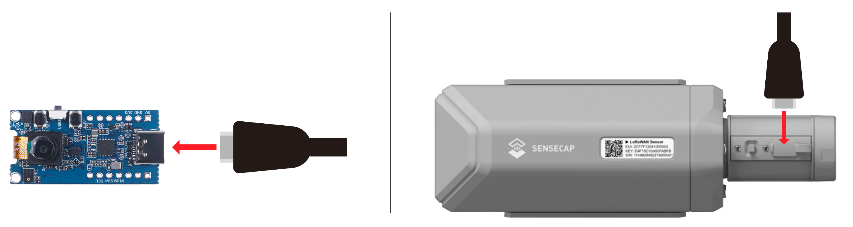
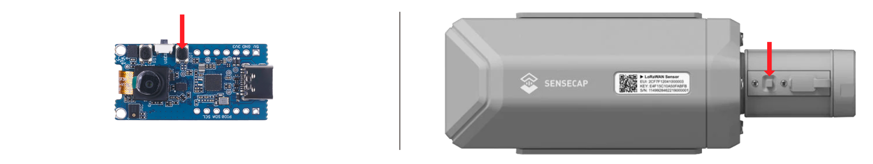
Step 1. Connect Grove - Vision AI Module/ SenseCAP A1101 to PC by using USB Type-C cable

Step 2. Double click the boot button to enter boot mode

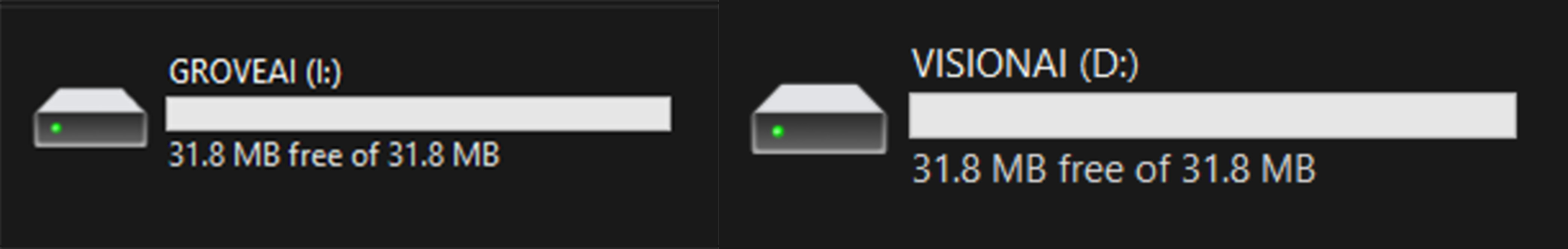
Step 3: After this you will see a new storage drive shown on your file explorer as GROVEAI for Grove - Vision AI Module and as VISIONAI for SenseCAP A1101

Step 4: Drag and drop the previous firmware.uf2 at first, and then the model.uf2 file to GROVEAI or VISIONAI

Once the copying is finished GROVEAI or VISIONAI drive will disapper. This is how we can check whether the copying is successful or not.

View live detection results

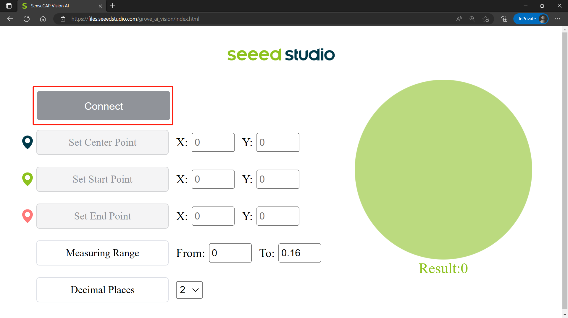
Step 1: After loading the firmware and connecting to PC, visit this URL
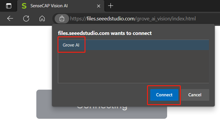
Step 2: Click Connect button. Then you will see a pop up on the browser. Select Grove AI - Paired and click Connect

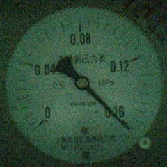
Upon successful connection, you will see a live preview from the camera. Here the camera is pointed at an analog meter.

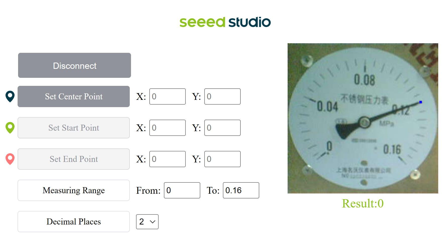
Now we need to set 3 points which is the center point, start point and the end point.

Step 3: Click on Set Center Point and click on the center of the meter. you will see a pop up confirm the location and press OK

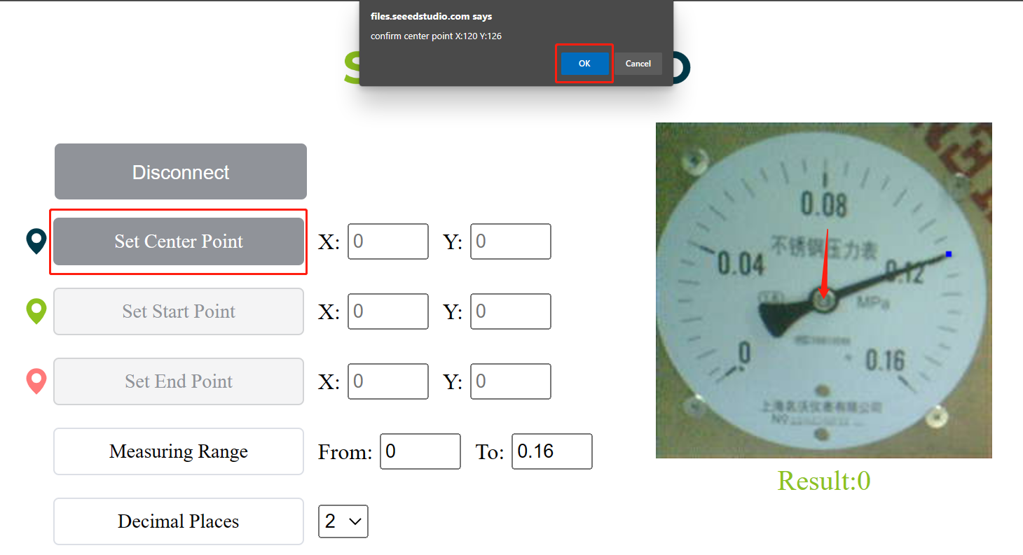
You will see the center point is already recorded

Step 4: Click on Set Start Point and click on the first indicator point. you will see a pop up confirm the location and press OK

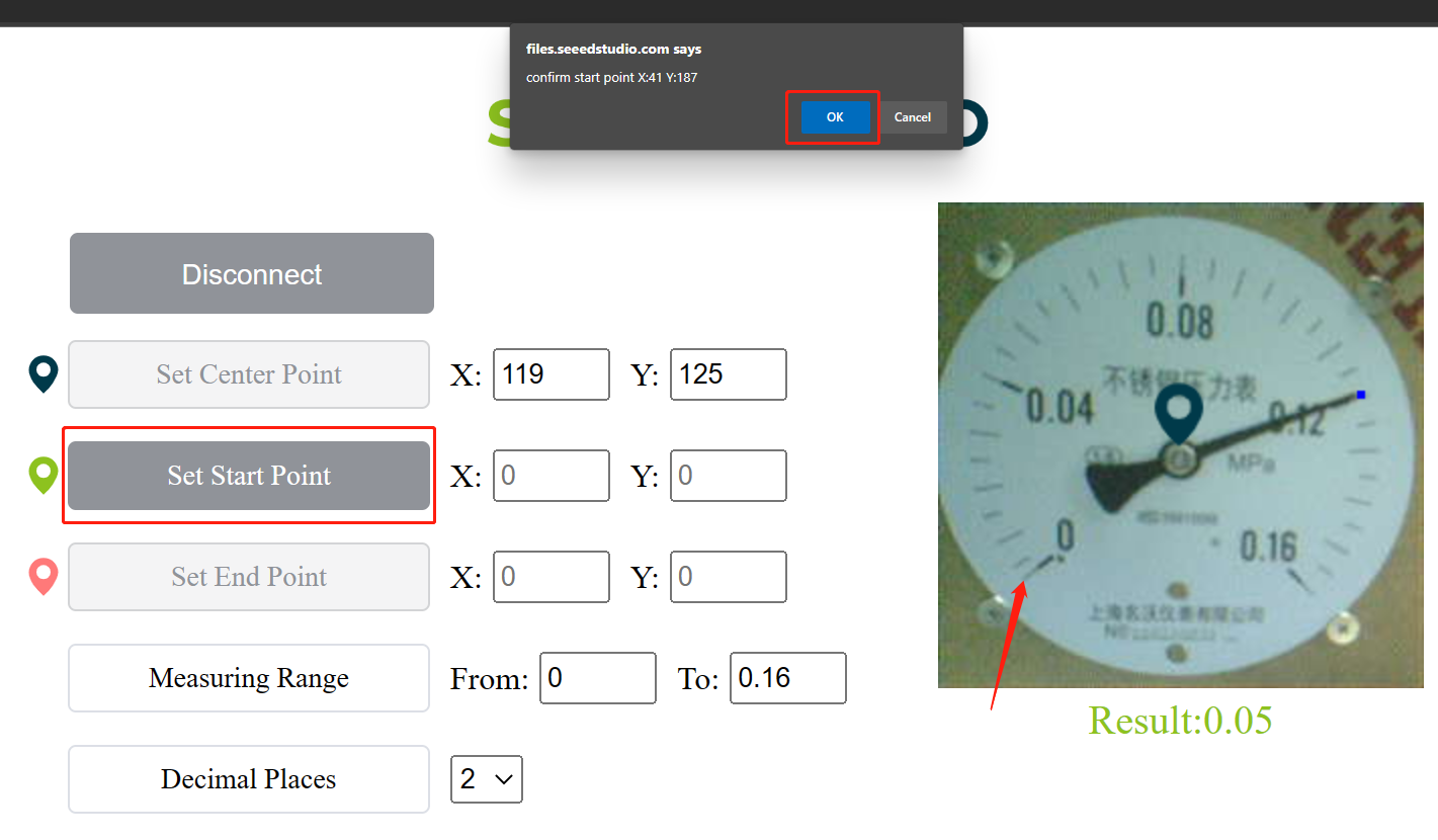
You will see the first indicator point is already recorded

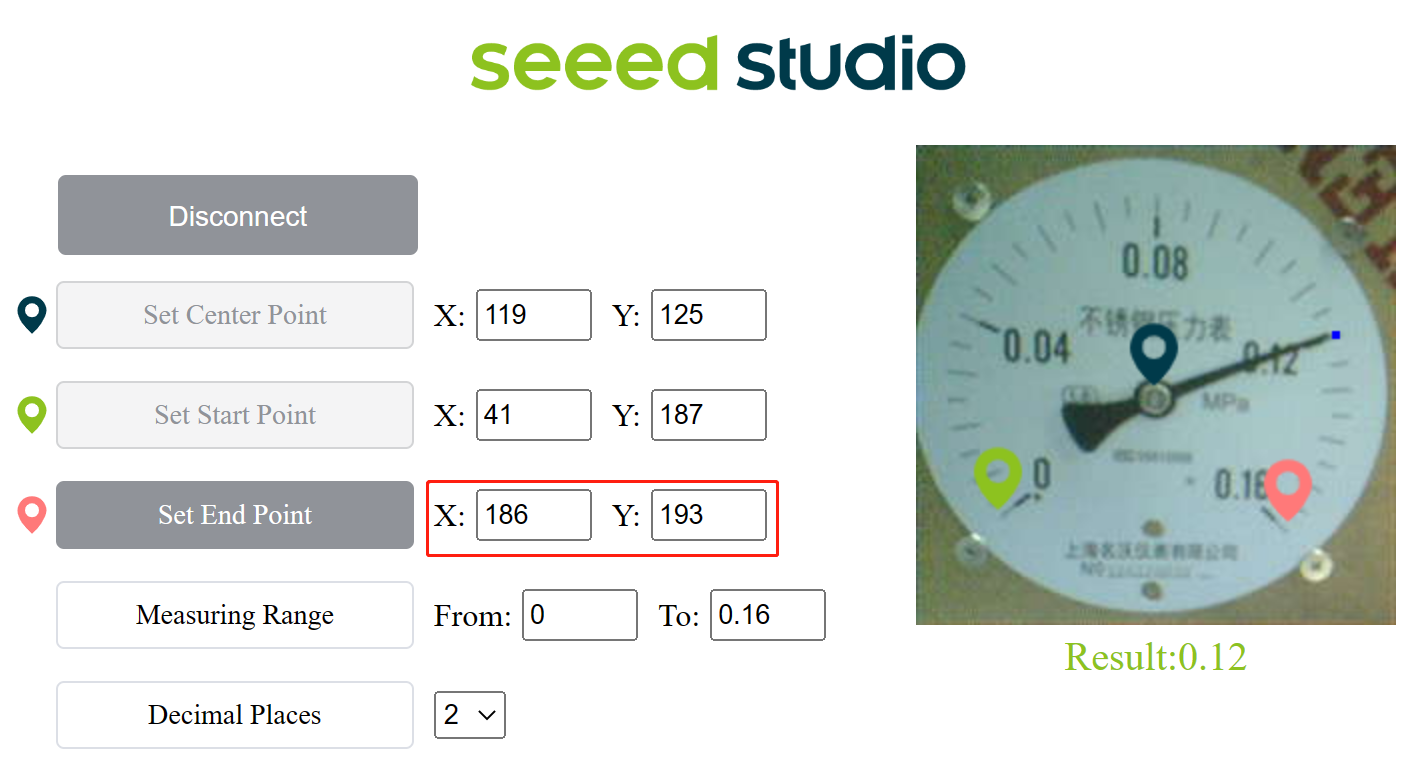
Step 5: Click on Set End Point and click on the last indicator point. you will see a pop up confirm the location and press OK

You will see the last indicator point is already recorded

Step 6: Set the measuring range according to the first digit and last digit of the meter. For example, he we set as From:0 To 0.16

Step 7: Set the number of decimal places that you want the result to display. Here we set as 2

Finally you can see the live meter reading results as follows

Files

Edgelab-getting-started.md

Latest commit

History

Edgelab-getting-started.md

File metadata and controls

Getting Started with EdgeLab on Local PC

1. Prerequisites

2. Configure host environment

3. Generate firmware image

Analog meter reading detection

Object Detection

4. Prepare dataset

Analog meter reading detection

With existing dataset

With your own dataset

Collect dataset

Pointer reading at dark environment

Pointer reading at light environment

Annotate dataset

Organize dataset

Object detection

With public dataset

Use PASCAL VOC dataset

Use other public datasets

With your own dataset

5. Start training

Configuration file

Analog meter reading detection

With existing dataset

With your own dataset

Object Detection

PASCAL VOC dataset

Other datasets (public/ own)

6. Export PyTorch to TFLite

Analog meter reading detection

Object detection

7. Convert TFLite to UF2

8. Deploy and Inference

Flash firmware and model

View live detection results